Intro to Probability Theory for Vision Science

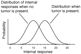
In this session, we’ll build your intuition for probability, the normal distribution, p-values, Type I/II errors, and statistical power — using examples rooted in clinical optometry. We'll even sketch some Gaussian curves along the way!

1. What is Probability?

Probability is a measure of uncertainty. In clinical work, we often ask things like:

• What is the chance this patient has glaucoma given a suspicious optic disc?
• How likely is it that this new contact lens reduces dryness symptoms?

Probability is a number between 0 and 1. If you flip a fair coin, the chance of heads is 0.5. If 60% of a population have a spherical equivalent (SE) below −0.50 D, then:

# Probability estimate in R
p_myopia <- 0.60
p_not_myopic <- 1 - p_myopia

2. The Normal Distribution

The normal distribution — aka the bell curve — is everywhere in vision science. It models things like intraocular pressure, visual acuity scores, and refractive errors.

# Simulate a normal distribution of refraction values
set.seed(123)
refraction <- rnorm(1000, mean = -1.00, sd = 1.5)
hist(refraction, breaks = 30, col = "lightblue", main = "Refraction in Young Adults", xlab = "Diopters")

• 68% of values fall within ±1 SD
• 95% within ±2 SD
• 99.7% within ±3 SD

3. p-values and Alpha (α)

The p-value is the probability of getting a result this extreme if the null hypothesis were true. A small p-value (typically < 0.05) suggests that your result is unlikely due to random chance.

# One-sample t-test: Is mean refraction different from emmetropia (0 D)?
t.test(refraction, mu = 0)

Alpha (α) is the threshold for a "rare" result. Usually, α = 0.05 (5%). That means:

• You’ll get a false positive 5% of the time if the null is true

4. Type I & II Errors (α and β)

Type I error (α): False positive
Type II error (β): False negative
Power: 1 − β — the probability you’ll detect a real effect when it exists.

5. Power and Sample Size

If you’re trying to detect a difference in refractive error, your ability to detect it depends on:

• Effect size (how big the difference is)
• Standard deviation
• Sample size
• Alpha

# Power analysis
library(pwr)
pwr.t.test(d = 0.5, power = 0.8, sig.level = 0.05, type = "two.sample")

6. Signal Detection Theory

Your visual system performs constant hypothesis testing: Is this edge real, or is it noise? Signal detection theory gives us:

• Hit: You detect the signal, and it's there
• Miss: You miss a real signal
• False Alarm: You detect something that's not there
• Correct Rejection: You correctly detect nothing

This is especially relevant in low-contrast vision tests or glaucoma screening.

Summary

• Probability helps you manage uncertainty.
• The normal distribution is key to understanding biological variation.
• p-values tell you if your results are rare, assuming the null is true.
• α and β define your error types — and power helps you detect real effects.

Frequentist vs Bayesian Thinking

Statisticians love to argue, and the most famous showdown is between Frequentist and Bayesian views of evidence.

Example: You test a new contact lens for reducing dryness.

• Frequentist: If dryness scores improved this much by chance alone (null is true), p = 0.03.
• Bayesian: Given what we know about similar lenses (prior) and our results, there's an 87% chance this lens is effective.

Frequentist vs Bayesian Inference

In this lab, you’ll compare traditional (Frequentist) and Bayesian approaches to evaluating evidence, using real-ish data from a sample of young adults with varying levels of myopia.

Question: Is the average spherical equivalent (SE) significantly different from emmetropia (0 D)?

Objectives

• Conduct a one-sample t-test using the Frequentist approach
• Perform a Bayesian t-test using prior knowledge
• Visualize and interpret a posterior distribution
• Compare how conclusions shift between methods

Setup

install.packages(c("BayesFactor", "ggplot2", "bayestestR"))

Part 1: Frequentist t-Test

We’ll use a one-sample t-test to see if the group’s mean SE differs from 0 D (emmetropia).

# Load and inspect data
df <- read.csv("myopia_study_data.csv")
summary(df$SE)

# Frequentist t-test
t.test(df$SE, mu = 0)

Part 2: Bayesian t-Test

This time, we ask: What is the probability that the true mean differs from 0 D, given our data and prior beliefs?

library(BayesFactor)

# Bayesian one-sample t-test
bf_result <- ttestBF(x = df$SE, mu = 0)
print(bf_result)

Interpret the Bayes Factor (BF₁₀):

• BF₁₀ < 1/3 → evidence for the null
• BF₁₀ ≈ 1 → inconclusive
• BF₁₀ > 3 → moderate evidence for a difference

Part 3: Visualizing the Posterior

Now let’s see what the Bayesian test thinks about the most credible values of the mean SE.

library(bayestestR)

# Visualize posterior
posterior <- estimate_density(bf_result)
plot(posterior, main = "Posterior Distribution of Mean SE")

# Highest Density Interval (HDI)
describe_posterior(bf_result)

Part 4: Interpretation and Reflection

• How do the Frequentist and Bayesian conclusions compare?
• Which feels more useful for a scientist trying to decide if students are "on average" myopic?
• How would a skeptical or optimistic prior change the Bayesian result?

Assignment Questions

1. Report the p-value and interpretation from the t-test.
2. Report the Bayes Factor and HDI.
3. Explain in plain English what the Bayesian result tells you that the p-value does not.
4. Would you advise clinicians differently depending on which method you used?

Bonus: Simulate a Study

# Simulate new sample with mild myopia
sim_data <- rnorm(40, mean = -0.75, sd = 1.2)

t.test(sim_data, mu = 0)
ttestBF(x = sim_data, mu = 0)

How does a smaller sample or effect size impact your inference? What does the Bayesian method still offer here?

Summary: Two Lenses for One Question

Both are useful. You’ll see them side by side in future research papers — so get comfy with both!